Package Overview
satpoint.RmdIn this article we will provide a worked example of using the
functions within the satpoint package to process netCDF
files. First, we will load some packages that will help with the
process.
netCDF files to process
If you are unsure how we can obtain netCDF files please see
vignette("download-netcdf", package = "satpoint"). We will
use the files downloaded there for this example.
nc_files <- list.files(pattern = ".nc4")
head(nc_files)
#> [1] "3B-DAY-L.MS.MRG.3IMERG.20200601-S000000-E235959.V07B.nc4"
#> [2] "3B-DAY-L.MS.MRG.3IMERG.20200602-S000000-E235959.V07B.nc4"
#> [3] "3B-DAY-L.MS.MRG.3IMERG.20200603-S000000-E235959.V07B.nc4"
#> [4] "3B-DAY-L.MS.MRG.3IMERG.20200604-S000000-E235959.V07B.nc4"
#> [5] "3B-DAY-L.MS.MRG.3IMERG.20200605-S000000-E235959.V07B.nc4"
#> [6] "3B-DAY-L.MS.MRG.3IMERG.20200606-S000000-E235959.V07B.nc4"
The Process
Sites
The satpoint package is designed to assist in extracting
values from netCDF files for particular areas. These areas can be
predefined by a user but we included a helper function to create
buffers around particular points, for example locations of fish
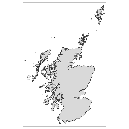
farms. In this example we construct a set of fake site locations,
sites <- tibble(
  site = LETTERS[1:4],
  longitude = c(-5.837704, -6.592514, -7.885055, -3.421410),
  latitude = c(57.607846, 57.291280, 56.900022, 58.187849)
)
sites
#> # A tibble: 4 × 3
#>   site  longitude latitude
#>   <chr>     <dbl>    <dbl>
#> 1 A         -5.84     57.6
#> 2 B         -6.59     57.3
#> 3 C         -7.89     56.9
#> 4 D         -3.42     58.2
which we can plot just for reference purposes.

Creating Buffer Zones
We can now create a set of circular buffers around these points, over
which we will average the values from the netCDF files. To do this we
use the site_buffers() function and specify that we want
10km, 15km and 20km buffers.
buffers <- site_buffers(sites, x_coord = "longitude", y_coord = "latitude", crs = 4326, buffers = c(10, 15, 20))
buffers
#> Simple feature collection with 12 features and 1 field
#> Geometry type: POLYGON
#> Dimension:     XY
#> Bounding box:  xmin: -8.218254 ymin: 56.71742 xmax: -3.076761 ymax: 58.36968
#> Geodetic CRS:  WGS 84
#> # A tibble: 12 × 2
#>    site                                                                      geometry
#>    <chr>                                                                <POLYGON [°]>
#>  1 A_10  ((-5.891903 57.52217, -5.889911 57.52227, -5.889591 57.52086, -5.887599 57.…
#>  2 B_10  ((-6.72602 57.23765, -6.725663 57.23627, -6.724667 57.23632, -6.724486 57.2…
#>  3 C_10  ((-7.840913 56.81297, -7.836937 56.81323, -7.832962 56.81348, -7.830974 56.…
#>  4 D_10  ((-3.585398 58.16313, -3.585212 58.1618, -3.584815 58.15896, -3.58333 58.15…
#>  5 A_15  ((-5.655942 57.51381, -5.656095 57.51452, -5.653116 57.51465, -5.649145 57.…
#>  6 B_15  ((-6.75816 57.19041, -6.757478 57.18778, -6.7535 57.188, -6.752773 57.1852,…
#>  7 C_15  ((-8.071833 56.81163, -8.071189 56.80955, -8.069197 56.80967, -8.068768 56.…
#>  8 D_15  ((-3.673967 58.16355, -3.673865 58.16284, -3.672874 58.16287, -3.672366 58.…
#>  9 A_20  ((-5.545368 57.51908, -5.545443 57.51943, -5.541972 57.51958, -5.542574 57.…
#> 10 B_20  ((-6.612155 57.47221, -6.612513 57.47361, -6.616525 57.4734, -6.620537 57.4…
#> 11 C_20  ((-8.182937 56.82204, -8.182502 56.82065, -8.180506 56.82079, -8.179201 56.…
#> 12 D_20  ((-3.218432 58.33415, -3.22215 58.33405, -3.222172 58.33423, -3.22242 58.33…
As above, we can plot these buffers to demonstrate what has been created.
Note: If you are creating your own buffer zones,
which do not have to be circular, the expectation is that the
buffers data frame will have a unique row per buffer and
these should have a unique identifier. In our case it is the
site column.
Extracting the Data
Now we have the buffers we can use the main package function
extract_site_grids_nc() to extract all the data values.
We’ll do this for one file first, to demonstrate the inputs and the
messages provided to help track the progress.
extract_site_grids_nc(nc_file = nc_files[1], sites = buffers, nc_crs = 4326)
#> Extracting the coordinate names directly from the file
#> Variable extracted from file is precipitation
#> Processing site A_10
#> Processing site A_15
#> Processing site A_20
#> Processing site B_10
#> Processing site B_15
#> Processing site B_20
#> Processing site C_10
#> Processing site C_15
#> Processing site C_20
#> # A tibble: 104 × 3
#>    site  precipitation datetime
#>    <chr>         <dbl> <dttm>
#>  1 A_10         0.125  2020-06-01 00:00:00
#>  2 A_10         0.415  2020-06-01 00:00:00
#>  3 A_10         0.440  2020-06-01 00:00:00
#>  4 A_10         0.0600 2020-06-01 00:00:00
#>  5 A_10         0      2020-06-01 00:00:00
#>  6 A_10         0      2020-06-01 00:00:00
#>  7 A_15         0.205  2020-06-01 00:00:00
#>  8 A_15         0.125  2020-06-01 00:00:00
#>  9 A_15         0.415  2020-06-01 00:00:00
#> 10 A_15         0.440  2020-06-01 00:00:00
#> # ℹ 94 more rows
As you can see, we must provide an netCDF file to process, the
buffers and the coordinate referencing system (CRS) that the netCDF file
is making use of. The extract_site_grids_nc() function
completes the following steps:
- open the netCDF file
- extract the date/time information from the file
- extract the geographic data from the file and establish which parts of the file intersect with the provided buffers
- extract the data from the netCDF file for the parts which intersect with the provided buffers
The result is a tibble with the site, data
value (in the above example precipitationCal) and the
datetime.
Processing all files
To demonstrate processing multiple files, we’ll use the
map() function to progress through all the input files and
bind the results together.
# Note that messages are hidden here to avoid a lot of repetition
precip <- map(nc_files, .f = extract_site_grids_nc,
              sites = buffers, nc_crs = 4326) %>%
  list_rbind()
precip
#> # A tibble: 3,120 × 3
#>    site  precipitation datetime
#>    <chr>         <dbl> <dttm>
#>  1 A_10         0.125  2020-06-01 00:00:00
#>  2 A_10         0.415  2020-06-01 00:00:00
#>  3 A_10         0.440  2020-06-01 00:00:00
#>  4 A_10         0.0600 2020-06-01 00:00:00
#>  5 A_10         0      2020-06-01 00:00:00
#>  6 A_10         0      2020-06-01 00:00:00
#>  7 A_15         0.205  2020-06-01 00:00:00
#>  8 A_15         0.125  2020-06-01 00:00:00
#>  9 A_15         0.415  2020-06-01 00:00:00
#> 10 A_15         0.440  2020-06-01 00:00:00
#> # ℹ 3,110 more rows
We can then summarise() the results and produce a quick
plot of them.
sum_precip <- precip %>%
  separate_wider_delim(site, names = c("site", "buffer"), delim = "_") %>%
  group_by(site, buffer, datetime) %>%
  summarise(precipitation = mean(precipitation, na.rm = TRUE),
            .groups = "drop")

ggplot(sum_precip, aes(x = datetime, y = precipitation)) +
  geom_line(aes(col = buffer)) +
  geom_point() +
  facet_grid(buffer ~ site) +
  labs(x = "Date", y = "Mean Precipitation", colour = "Buffer")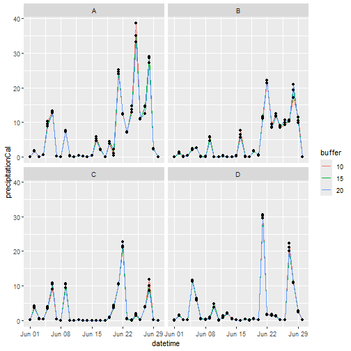
Additional Options
Extracting Certain Dates
In the example above, each netCDF file only contained a single days
worth of data. Other netCDF files can contain months or years worth of
data. In those cases, a date or dates can be provided to the
extract_site_grids_nc() function and only data for that
date(s) will be returned. For example:
# not run
extract_site_grids_nc(nc_file = nc_files[1], site_buffers = buffers, nc_crs = 4326,
                      dates_to_extract = c("2023-01-01", "2024-01-01"))
# or with a pre-defined sequence of dates
date_seq <- seq.Date(as.Date("2023-01-01"), as.Date("2023-01-04"), by = "day")
extract_site_grids_nc(nc_file = nc_files[1], site_buffers = buffers, nc_crs = 4326,
                      dates_to_extract = date_seq)
If a particular date(s), requested in dates_to_extract
is not present in the data, a message will be printed out specifying the
missing date(s).
Extracting Certain Depths
Where a netCDF file has multiple depths, a (numerical) vector of depths to extract can be provide and then only these depths will be returned. If none of the depths provided match those in the file, all depths will be returned.
For example - if the file contains depth values of 0, 5, 10 and 15 we can return only the first two values
# not run
extract_site_grids_nc(nc_file = nc_files[1], site_buffers = buffers, nc_crs = 4326,
                      depths_to_extract = c(0, 5))
or just the value at 10m.
# not run
extract_site_grids_nc(nc_file = nc_files[1], site_buffers = buffers, nc_crs = 4326,
                      depths_to_extract = 10)
Providing details on the variables to extract
By default extract_site_grids_nc() will try its best to
figure out which variable to extract. However, if this can be specified
via the
# not run
extract_site_grids_nc(nc_file = nc_files[1], site_buffers = buffers, nc_crs = 4326,
                      nc_var_name = "precipitation")
#> Error in extract_site_grids_nc(nc_file = nc_files[1], site_buffers = buffers, : unused argument (site_buffers = buffers)
Likewise, where a depth variable is present, the function will try to extract the details automatically but the variable name can also be extracted.
# not run
extract_site_grids_nc(nc_file = nc_files[1], site_buffers = buffers, nc_crs = 4326,
                      nc_var_name = "precipitation", depth_var = "Depth")